1. Model initialization and selection procedure
In this notebook, we will show how CoPro is initialized and the selection procedure of spatial aggregation units and conflicts works.
1.1. Model initialization
Start with loading the required packages.
[1]:
from copro import utils, selection, plots, data

%matplotlib inline

import matplotlib.pyplot as plt
import numpy as np
import seaborn as sns
import os, sys
import warnings
warnings.simplefilter("ignore")
For better reproducibility, the version numbers of all key packages used to run this notebook are provided.
[2]:
utils.show_versions()
Python version: 3.7.8 | packaged by conda-forge | (default, Jul 31 2020, 01:53:57) [MSC v.1916 64 bit (AMD64)]
copro version: 0.0.8
geopandas version: 0.9.0
xarray version: 0.15.1
rasterio version: 1.1.0
pandas version: 1.0.3
numpy version: 1.18.1
scikit-learn version: 0.23.2
matplotlib version: 3.2.1
seaborn version: 0.11.0
rasterstats version: 0.14.0
1.2. The configurations-file (cfg-file)
In the configurations-file (cfg-file), all the settings for the analysis are defined. The cfg-file contains, amongst others, all paths to input files, settings for the machine-learning model, and the various selection criteria for spatial aggregation units and conflicts. Note that the cfg-file can be stored anywhere, not per se in the same directory where the model data is stored (as in this example case). Make sure that the paths in the cfg-file are updated if you use relative paths and change the folder location of th cfg-file!
[3]:
settings_file = 'example_settings.cfg'
Based on this cfg-file, the set-up of the run can be initialized. Here, the cfg-file is parsed (i.e. read) and all settings and paths become ‘known’ to the model. Also, the output folder is created (if it does not exist yet) and the cfg-file is copied to the output folder for improved reusability.
If you set verbose=True, then additional statements are printed during model execution. This can help to track the behaviour of the model.
[4]:
main_dict, root_dir = utils.initiate_setup(settings_file, verbose=False)
#### CoPro version 0.0.8 ####
#### For information about the model, please visit https://copro.readthedocs.io/ ####
#### Copyright (2020-2021): Jannis M. Hoch, Sophie de Bruin, Niko Wanders ####
#### Contact via: j.m.hoch@uu.nl ####
#### The model can be used and shared under the MIT license ####

INFO: reading model properties from example_settings.cfg
INFO: verbose mode on: False
INFO: saving output to main folder C:\Users\hoch0001\Documents\_code\copro\example\./OUT
One of the outputs is a dictionary (here main_dict) containing the parsed configurations (they are stored in computer memory, therefore the slighly odd specification) as well as output directories of both the reference run and the various projection runs specified in the cfg-file.
For the reference run, only the respective entries are required.
[5]:
config_REF = main_dict['_REF'][0]
print('the configuration of the reference run is {}'.format(config_REF))
out_dir_REF = main_dict['_REF'][1]
print('the output directory of the reference run is {}'.format(out_dir_REF))
the configuration of the reference run is <configparser.RawConfigParser object at 0x000001FBC8FA9D08>
the output directory of the reference run is C:\Users\hoch0001\Documents\_code\copro\example\./OUT\_REF
1.3. Filter conflicts and spatial aggregation units
1.3.1. Background
As conflict database, we use the UCDP Georeferenced Event Dataset. Not all conflicts of the database may need to be used for a simulation. This can be, for example, because they belong to a non-relevant type of conflict we are not interested in, or because it is simply not in our area-of-interest. Therefore, it is possible to filter the conflicts on various properties:
min_nr_casualties: minimum number of casualties of a reported conflict;
type_of_violence: 1=state-based armed conflict; 2=non-state conflict; 3=one-sided violence.
To unravel the interplay between climate and conflict, it may be beneficial to run the model only for conflicts in particular climate zones. It is hence also possible to select only those conflcits that fall within a climate zone following the Koeppen-Geiger classification.
1.3.2. Selection procedure
In the selection procedure, we first load the conflict database and convert it to a georeferenced dataframe (geo-dataframe). To define the study area, a shape-file containing polygons (in this case water provinces) is loaded and converted to geo-dataframe as well.
We then apply the selection criteria (see above) as specified in the cfg-file, and keep the remaining data points and associated polygons.
[7]:
conflict_gdf, selected_polygons_gdf, global_df = selection.select(config_REF, out_dir_REF, root_dir)
INFO: reading csv file to dataframe C:\Users\hoch0001\Documents\_code\copro\example\./example_data\UCDP/ged201.csv
INFO: filtering based on conflict properties.
With the chosen settings, the following picture of polygons and conflict data points is obtained.
[8]:
fig, ax= plt.subplots(1, 1, figsize=(20,10))
conflict_gdf.plot(ax=ax, c='r', column='best', cmap='magma',
                  vmin=int(config_REF.get('conflict', 'min_nr_casualties')), vmax=conflict_gdf.best.mean(),
                  legend=True,
                  legend_kwds={'label': "# casualties", 'orientation': "vertical", 'pad': 0.05})
selected_polygons_gdf.boundary.plot(ax=ax);
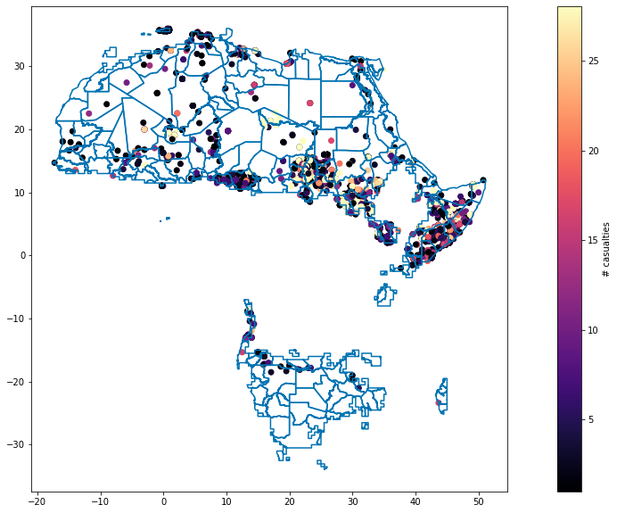
It’s nicely visible that for this example-run, not all provinces are considered but we focus on specified climate zones only.
1.4. Temporary files
To be able to also run the following notebooks, some of the data has to be written to file temporarily. This is not part of the CoPro workflow but merely needed to split up the workflow in different notebooks outlining the main steps to go through when using CoPro.
[9]:
if not os.path.isdir('temp_files'):
        os.makedirs('temp_files')
[10]:
conflict_gdf.to_file(os.path.join('temp_files', 'conflicts.shp'))
selected_polygons_gdf.to_file(os.path.join('temp_files', 'polygons.shp'))
[11]:
global_df['ID'] = global_df.index.values
global_arr = global_df.to_numpy()
np.save(os.path.join('temp_files', 'global_df'), global_arr)